Numerical implementation of the optimized explicit solver for elastodynamics problems#
Authors: A. Chao Correas (arturo.chaocorreas@polito.it) and C. Maurini (corrado.maurini@sorbonne-universite.fr)
The libraries here required are the same as those used in the Elastodynamics-Implementation notebook, with which this notebook shares a lot of features. As a consequence, only the differences will be commented.
import logging
import ipyparallel as ipp

# create a cluster
rc = ipp.Cluster(engines="mpi", n=2, log_level=logging.INFO).start_and_connect_sync(activate=True)
Starting 2 engines with <class 'ipyparallel.cluster.launcher.MPIEngineSetLauncher'>
%%px

import dolfinx, ufl
import numpy as np
import sympy as sp
from mpi4py import MPI
from petsc4py import PETSc
from matplotlib import pyplot as plt
import sys
#import mesh_plotter
import dolfinx.fem.petsc


sys.path.append("../utils/")
from petsc_problems import SNESProblem

comm = MPI.COMM_WORLD
In what concerns the input parameters, only those relative to the time stepping present some differences. Due to the necessity to comply with the CFL condition to keep stability in the solution, the present implementation does not take delta_t0 as an input but it calculates the critical time increment delta_t_critical based on the material properties and the mesh characteristics. Then, the time increment delta_t0 is set as delta_t_critical/explicit_safety_factor, where it is advised that the latter is reasonably higher than 1.
%%px

# Characteristic dimensions of the domain
geometry_parameters = {'Lx': 1.,
                       'Ly': 0.1}

# Regularization length
material_properties = {'E':   3e3,
                       'nu':  0.3,
                       'rho': 1.8e-9,
                       'c1':  1e-5,
                       'c2':  5e-5}

# Mesh control
mesh_parameters = {'nx': 10,
                   'ny': 1}

# Time stepping control
timestepping_parameters = {'initial_time':0.,
                           'total_time':20e-6,
                           'explicit_safety_factor': 5}

# Output parameters
OTP_settings = {'xdmf_filename': f"explicit_elastodynamics.xdmf"}

# Top facet displacement
T_0 = 0.
T_1 = 2.5e-6
U_t = 1e-2

t_sp = sp.Symbol('t', real = True)
U_imp = sp.Piecewise((0, t_sp<T_0),
                     (0.5*U_t*(1-sp.cos(((t_sp-T_0)/(T_1-T_0))*sp.pi)), t_sp<=T_1),
                     (U_t, True))
V_imp = sp.diff(U_imp, t_sp)
A_imp = sp.diff(V_imp, t_sp)

# Body forces
b_ = np.asarray([0.,0.])
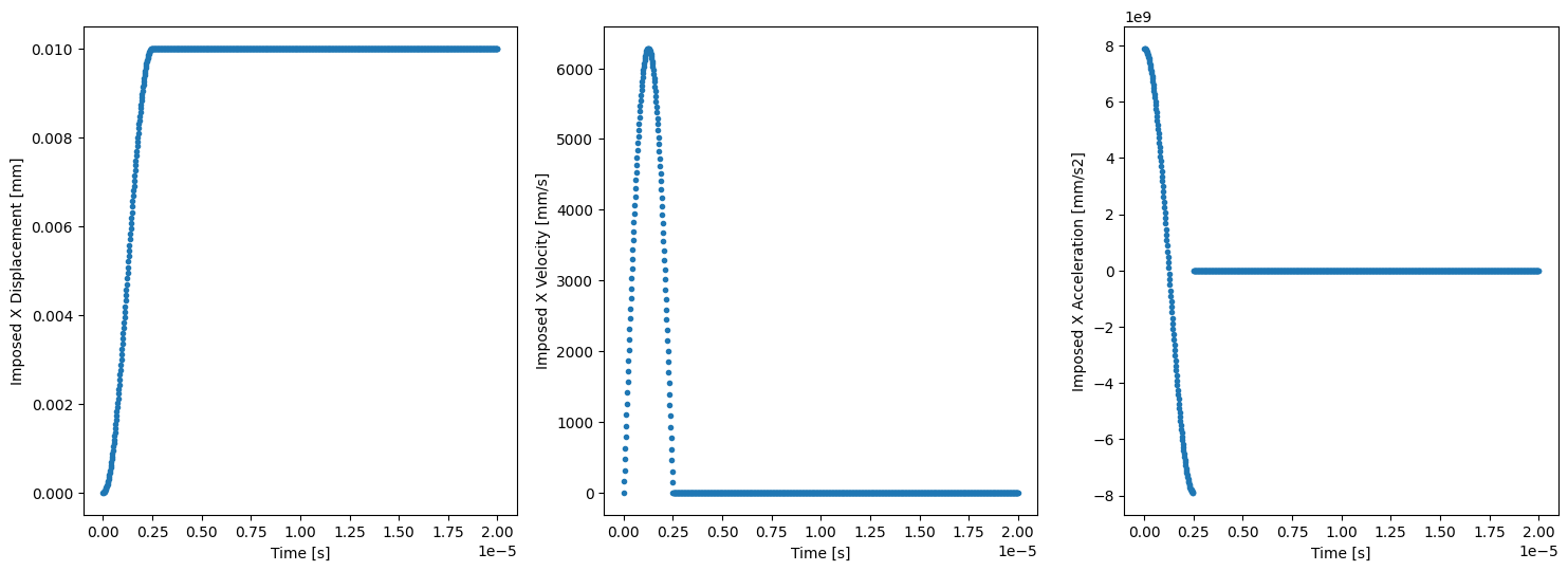
The loading and mesh here implemented are equivalent to those in the Elastodynamics-Implementation notebook
%%px

if comm.rank == 0:
    t_sampling = np.linspace(timestepping_parameters['initial_time'],
                             timestepping_parameters['total_time'],
                             1000)
    U_imp_sampling = np.zeros_like(t_sampling)
    V_imp_sampling = np.zeros_like(t_sampling)
    A_imp_sampling = np.zeros_like(t_sampling)

    for i in enumerate (t_sampling):
        U_imp_sampling[i[0]] = U_imp.subs({t_sp:t_sampling[i[0]]})
        V_imp_sampling[i[0]] = V_imp.subs({t_sp:t_sampling[i[0]]})
        A_imp_sampling[i[0]] = A_imp.subs({t_sp:t_sampling[i[0]]})

    fig, ax = plt.subplots(1, 3, figsize=(18,6))
    ax[0].plot(t_sampling, U_imp_sampling, ls='none', marker='.')
    ax[0].set_xlabel('Time [s]')
    ax[0].set_ylabel('Imposed X Displacement [mm]')
    ax[1].plot(t_sampling, V_imp_sampling, ls='none', marker='.')
    ax[1].set_xlabel('Time [s]')
    ax[1].set_ylabel('Imposed X Velocity [mm/s]')
    ax[2].plot(t_sampling, A_imp_sampling, ls='none', marker='.')
    ax[2].set_xlabel('Time [s]')
    ax[2].set_ylabel('Imposed X Acceleration [mm/s2]');
[output:0]
%%px

mesh = dolfinx.mesh.create_rectangle(MPI.COMM_WORLD,
                                     [np.array([-geometry_parameters['Lx']/2, -geometry_parameters['Ly']/2]),
                                      np.array([+geometry_parameters['Lx']/2, +geometry_parameters['Ly']/2])],
                                     [mesh_parameters['nx'], mesh_parameters['ny']],
                                     dolfinx.mesh.CellType.triangle)
gdim = mesh.topology.dim
fdim = gdim - 1
# mesh_plotter(mesh)
As explained in the Elastodynamics_Explicit-Theory the CFL condition for an explicit elastodynamics solver is based on the minimum distance between nodes in the mesh. Nonetheless, and to the best of our knowledge, dolfinx:v0.6.0-r1 does not have a built-in function that calculates the minimum distance between nodes in an element, yet the maximum counterpart can be determined using dolfinx.cpp.mesh.h. Hence, given that the elements here implemented are not distorted, and considering the safety factor used for the CFL condition, the minimum in the domain of the maximum distance between two nodes of an element is hereafter used as h_min without compromising the stability of the solution.
%%px
tdim = mesh.topology.dim
h_min_local= min(mesh.h(tdim, np.arange(mesh.topology.index_map(tdim).size_local, dtype=np.int32))) #Minimum internodal distance h of every processor submesh
h_min = np.asarray(comm.gather(h_min_local, root=0)) # Gather the minimum internodal distance of every processor submesh in an array at processor 0
if comm.rank == 0:  #Calculate the global minimum of h at processor 0
    h_min = min(h_min)
h_min = MPI.COMM_WORLD.bcast(h_min, root=0) #Broadcast to every processor the global minimum of h.
%%px

# Geometrical regions
def top(x):
    return np.isclose(x[1], +geometry_parameters["Ly"]/2)
def bottom(x):
    return np.isclose(x[1], -geometry_parameters["Ly"]/2)
def right (x):
    return np.isclose(x[0], +geometry_parameters["Lx"]/2)
def left (x):
    return np.isclose(x[0], -geometry_parameters["Lx"]/2)

# Geometrical sets
top_facets    = dolfinx.mesh.locate_entities_boundary(mesh, fdim, top)
bottom_facets = dolfinx.mesh.locate_entities_boundary(mesh, fdim, bottom)
right_facets  = dolfinx.mesh.locate_entities_boundary(mesh, fdim, right)
left_facets   = dolfinx.mesh.locate_entities_boundary(mesh, fdim, left)

tagged_facets = np.hstack([top_facets,
                           bottom_facets,
                           right_facets,
                           left_facets])

tag_values = np.hstack([np.full_like(top_facets,    1),
                        np.full_like(bottom_facets, 2),
                        np.full_like(right_facets,  3),
                        np.full_like(left_facets,   4)])

tagged_facets_sorted = np.argsort(tagged_facets)

mt = dolfinx.mesh.meshtags(mesh, fdim,
                           tagged_facets[tagged_facets_sorted],
                           tag_values[tagged_facets_sorted])

# Domain and subdomain measures
dx  = ufl.Measure("dx", domain=mesh)                         # Domain measure
ds  = ufl.Measure("ds", domain=mesh, subdomain_data=mt)      # External Boundary measure
dS  = ufl.Measure("dS", domain=mesh, subdomain_data=mt)      # External/Internal measure
n   = ufl.FacetNormal(mesh)                                  # External normal to the boundary
At this point, we have to also include a vector field ones_a which stores the unit nodal acceleration vector required for lumping the Consistent Mass matrix. Despite it being constant in value (and equal to (1,1)) all along the domain, a dolfinx.fem.function (and not a dolfinx.fem.Constant) must be used, as explained afterwards.
%%px

# --------- Main functions and function spaces
V_t = dolfinx.fem.functionspace(mesh, ("Lagrange", 1, (2,)))
u = dolfinx.fem.Function(V_t, name="Displacement")
u_new = dolfinx.fem.Function(V_t)
v = dolfinx.fem.Function(V_t, name="Velocity")
v_new = dolfinx.fem.Function(V_t)
a = dolfinx.fem.Function(V_t, name="Acceleration")
a_new = dolfinx.fem.Function(V_t)

# --------- Unit nodal acceleration
ones_a = dolfinx.fem.Function(V_t)

# --------- State of each field
state     = {"u": u,
             "v": v,
             "a": a}
state_new = {"u_new": u_new,
             "v_new": v_new,
             "a_new": a_new}
%%px

# Clamped left (ux=uy=0, vx=vy=0, ax=ay=0)
left_u = dolfinx.fem.Constant(mesh, PETSc.ScalarType((0,0)))
left_v = dolfinx.fem.Constant(mesh, PETSc.ScalarType((0,0)))
left_a = dolfinx.fem.Constant(mesh, PETSc.ScalarType((0,0)))
blocked_dofs_left_Vt = dolfinx.fem.locate_dofs_topological(V_t, fdim, left_facets)
bc_u_left = dolfinx.fem.dirichletbc(left_u, blocked_dofs_left_Vt, V_t)
bc_v_left = dolfinx.fem.dirichletbc(left_v, blocked_dofs_left_Vt, V_t)
bc_a_left = dolfinx.fem.dirichletbc(left_a, blocked_dofs_left_Vt, V_t)

# Imposed displacement right (ux=U_imp(t), vx=U_imp'(t), ax=U_imp''(t))
right_ux = dolfinx.fem.Constant(mesh,PETSc.ScalarType(0))
right_vx = dolfinx.fem.Constant(mesh,PETSc.ScalarType(0))
right_ax = dolfinx.fem.Constant(mesh,PETSc.ScalarType(0))
right_boundary_dofs_Vtx = dolfinx.fem.locate_dofs_topological(V_t.sub(0), fdim, right_facets)
bc_ux_right = dolfinx.fem.dirichletbc(right_ux, right_boundary_dofs_Vtx, V_t.sub(0))
bc_vx_right = dolfinx.fem.dirichletbc(right_vx, right_boundary_dofs_Vtx, V_t.sub(0))
bc_ax_right = dolfinx.fem.dirichletbc(right_ax, right_boundary_dofs_Vtx, V_t.sub(0))

# Collect the BCs
bcs_u = [bc_u_left, bc_ux_right]
bcs_v = [bc_v_left, bc_ux_right]
bcs_a = [bc_a_left, bc_ax_right]
%%px

t       = dolfinx.fem.Constant(mesh, PETSc.ScalarType(0))
delta_t = dolfinx.fem.Constant(mesh, PETSc.ScalarType(0))

# Material properties
E   = dolfinx.fem.Constant(mesh, PETSc.ScalarType(1))
nu  = dolfinx.fem.Constant(mesh, PETSc.ScalarType(0))
rho = dolfinx.fem.Constant(mesh, PETSc.ScalarType(1))
c1  = dolfinx.fem.Constant(mesh, PETSc.ScalarType(0))
c2  = dolfinx.fem.Constant(mesh, PETSc.ScalarType(0))

# Body forces
b = dolfinx.fem.Constant(mesh, PETSc.ScalarType((0,0)))

## Kinetic energy density
kinetic_energy_density = 0.5 * rho * ufl.inner(v,v)

### Dissipated energy density
eps_v = ufl.variable(ufl.sym(ufl.grad(v)))
dissipated_power_density = 0.5 * (c1 * ufl.inner(v,v) + c2 * ufl.inner(eps_v,eps_v))

# Lame constants (Plane strain)
mu    = E / (2.0 * (1.0 + nu))
lmbda = E * nu / ((1.0 + nu) * (1.0 - 2.0 * nu))

## Infinitesimal strain tensor
eps = ufl.variable(ufl.sym(ufl.grad(u)))

## Strain energy density (Linear elastic)
elastic_energy_density = lmbda / 2 * ufl.tr(eps) ** 2 + mu * ufl.inner(eps,eps)

# Stress tensor
sigma = ufl.diff(elastic_energy_density, eps) + c2*eps_v

## External workd density
external_work_density = ufl.dot(b,u)

# System's energy components
kinetic_energy   = kinetic_energy_density * dx
dissipated_power = dissipated_power_density * dx
elastic_energy   = elastic_energy_density * dx
external_work    = external_work_density * dx

potential_energy = elastic_energy - external_work
total_energy     = kinetic_energy + potential_energy

# Energy derivatives
u_test = ufl.TestFunction(V_t)
P_du = ufl.derivative(potential_energy, u, u_test)
K_dv = ufl.derivative(kinetic_energy,   v, u_test)
Q_dv = ufl.derivative(dissipated_power, v, u_test)

# Residual
Res = ufl.replace(K_dv, {v: a}) + Q_dv + P_du
Once defined the variational formulation of the problem, the obtention of the Consistent M and Lumped M_lumped mass matrices can be taken forward. In particular, the former can be directly determined by taking the bilinear form within K_dv, which can be achieved by using ufl.lhs. The ufl.replace is used to ensure that the proper Trial and Test functions of V_t will be used to compute the bilinear form.
Then, the form of the lumped mas matrix M_lumped_form is defined using the ufl.action instruction so that the former is the result of the action of M (a bilinear form) over ones_a (a linear form). Dur to this ones_a cannot be defined as a dolfinx.fem.Constant. This implies that M_lumped_form is also a linear form.
In matricial notation, this latter instruction is equivalent to the mathematical expression:
where \(\underline{M_l}\) is the diagonal of the Lumped Mass matrix \(\underline{\underline{M_l}}\) defined in 03-Elastodynamics_Explicit-Theory.
At the same time, the linear form of the nodal forces \(\underline{F}\) is assigned to F_form.
%%px

M = ufl.lhs(ufl.replace(K_dv,{v: ufl.TrialFunction(V_t)}))
M_lumped_form = dolfinx.fem.form(ufl.action(M, ones_a))
F_form = dolfinx.fem.form(ufl.replace(-(P_du+Q_dv),{u:u_new}))
%%px

# Magnitudes of interest
kinetic_energy_form       = dolfinx.fem.form(kinetic_energy)
dissipated_power_form     = dolfinx.fem.form(dissipated_power)
elastic_energy_form       = dolfinx.fem.form(elastic_energy)
potential_energy_form     = dolfinx.fem.form(potential_energy)
total_energy_form         = dolfinx.fem.form(potential_energy + kinetic_energy)
reaction_force_right_form = dolfinx.fem.form(ufl.inner(n,sigma*n)*ds(3))
In what concerns the iterative resolution of the problem, there exists major differences with the implicit elastodynamics solver, as it was shown in 03-Elastodynamics_Explicit-Theory notebook. Nonetheless, focusing only on the computational aspect of the differences, the main aspect to point out concerns the computation of the Lumped Mass matrix and the vector of nodal forces.
Firstly, as previously stated, M_lumped_form is a linear form and not a bilinear one, and thus it is associated with a vector, and not a matrix. Nonetheless, for the Lumped Mass matrix is diagonal it can be treated as a vector instead without any loss of information. In such a case, the matrix-vector multiplication and matrix inversion operations are substituted by component-wise vector-vector multiplication and component-wise inversion, respectively. The combination of both aforementioned operations is done using petsc.pointwiseDivide function.
Besides, given that the system here considered is assumed to not change its mass ditribution with time, the computation of the Lumped Mass “vector” M_lumped can be done just once before the time stepping, for it will remain constant all along the simulation time. On the other hand, the vector of nodal forces F must be computed at each time step for it varies from instant to instant. In order to keep the memory requirements low, F is destroyed once it is no longer needed at each time step.
%%px

# Initialization
t0         = timestepping_parameters['initial_time']
total_time = timestepping_parameters["total_time"]
explicit_safety_factor = timestepping_parameters["explicit_safety_factor"]

E.value   = material_properties["E"]
nu.value  = material_properties["nu"]
rho.value = material_properties["rho"]
c1.value  = material_properties["c1"]
c2.value  = material_properties["c2"]

b.value = b_

t.value = t0

for const in [left_u,left_v,left_a]:
    const.value = (0.,0.)

for func in [u,v,a] :
    func.x.array[:] = 0.

ones_a.x.array[:] = 1.

stp_cont = 0
ts = []
kinetic_energies       = []
dissipated_energies    = []
dissipated_energy      = 0
elastic_energies       = []
external_works         = []
potential_energies     = []
reaction_force_right_s = []

M_lumped = dolfinx.fem.petsc.assemble_vector(M_lumped_form)
M_lumped.ghostUpdate(addv=PETSc.InsertMode.ADD, mode=PETSc.ScatterMode.REVERSE)
M_lumped.ghostUpdate(addv=PETSc.InsertMode.INSERT, mode=PETSc.ScatterMode.FORWARD)

# Critical time increment (approximated CFL condition)
c = np.sqrt((E.value/rho.value)*((1-nu.value)/((1+nu.value)*(1-2*nu.value))))
delta_t_critic = h_min/c
delta_t0 = delta_t_critic/explicit_safety_factor
delta_t.value = delta_t0

with dolfinx.io.XDMFFile(comm,'tmp.xdmf','w') as xdmf_file:
    xdmf_file = dolfinx.io.XDMFFile(mesh.comm, OTP_settings['xdmf_filename'], "w")
    xdmf_file.write_mesh(mesh)
    xdmf_file.write_function(u, t.value)

if comm.rank == 0:
    print ('RESOLUTION STATUS')
    sys.stdout.flush()

while float(t.value) < total_time:

    #if comm.rank == 0:
    #    print(f"Solving for t = {t.value}")
    #    sys.stdout.flush()

    right_ux.value = float(U_imp.subs({t_sp:t.value}))
    right_vx.value = float(V_imp.subs({t_sp:t.value}))
    right_ax.value = float(A_imp.subs({t_sp:t.value}))

    #Update displacement field
    u_new.x.array[:] = u.x.array + delta_t*v.x.array + 0.5*delta_t**2*a.x.array
    dolfinx.fem.set_bc(u_new.x.petsc_vec,bcs_u)
    u_new.x.petsc_vec.ghostUpdate(addv=PETSc.InsertMode.INSERT, mode=PETSc.ScatterMode.FORWARD)

    # Update acceleration
    F = dolfinx.fem.petsc.assemble_vector(F_form)
    F.ghostUpdate(addv=PETSc.InsertMode.ADD, mode=PETSc.ScatterMode.REVERSE)
    F.ghostUpdate(addv=PETSc.InsertMode.INSERT, mode=PETSc.ScatterMode.FORWARD)

    a_new.x.petsc_vec.pointwiseDivide(F, M_lumped)
    a_new.x.petsc_vec.ghostUpdate(addv=PETSc.InsertMode.INSERT, mode=PETSc.ScatterMode.FORWARD)
    dolfinx.fem.set_bc(a_new.x.petsc_vec,bcs_a)
    a_new.x.petsc_vec.ghostUpdate(addv=PETSc.InsertMode.INSERT, mode=PETSc.ScatterMode.FORWARD)
    F.destroy()

    # Update velocity
    v_new.x.array[:] = v.x.array + 0.5*delta_t*(a_new.x.array + a.x.array)
    dolfinx.fem.set_bc(v_new.x.petsc_vec,bcs_v)
    v_new.x.petsc_vec.ghostUpdate(addv=PETSc.InsertMode.INSERT, mode=PETSc.ScatterMode.FORWARD)

     # Copy i+1 into i
    u.x.array[:] = u_new.x.array
    v.x.array[:] = v_new.x.array
    a.x.array[:] = a_new.x.array

    dissipated_energy += float(comm.allreduce(float(delta_t)*dolfinx.fem.assemble_scalar(dissipated_power_form), op=MPI.SUM))

    t.value += float(delta_t)
    delta_t.value = float(ufl.conditional(ufl.lt(delta_t0,total_time-t),
                                                 delta_t0,
                                                 total_time - t))

    kinetic_energies = np.concatenate((kinetic_energies,
                             [comm.allreduce(dolfinx.fem.assemble_scalar(kinetic_energy_form), op=MPI.SUM)]))
    dissipated_energies = np.concatenate((dissipated_energies,[dissipated_energy]))
    elastic_energies = np.concatenate((elastic_energies,
                            [comm.allreduce(dolfinx.fem.assemble_scalar(elastic_energy_form), op=MPI.SUM)]))
    potential_energies = np.concatenate((elastic_energies,
                            [comm.allreduce(dolfinx.fem.assemble_scalar(potential_energy_form), op=MPI.SUM)]))
    reaction_force_right_s = np.concatenate((reaction_force_right_s,
                            [comm.allreduce(dolfinx.fem.assemble_scalar(reaction_force_right_form), op=MPI.SUM)]))
    ts = np.concatenate((ts,[t.value]))

    #with dolfinx.io.XDMFFile(comm,OTP_settings['xdmf_filename'],'a') as xdmf_file:
    #    xdmf_file.write_function(u, t.value)

    if comm.rank == 0:
        if stp_cont != round((100*t.value/total_time)):
            stp_cont = round((100*t.value/total_time))
            print (f"="*stp_cont+"> "+str(stp_cont)+"%", end="\r")
            sys.stdout.flush()
[stdout:0] RESOLUTION STATUS
====================================================================================================> 100%
%%px
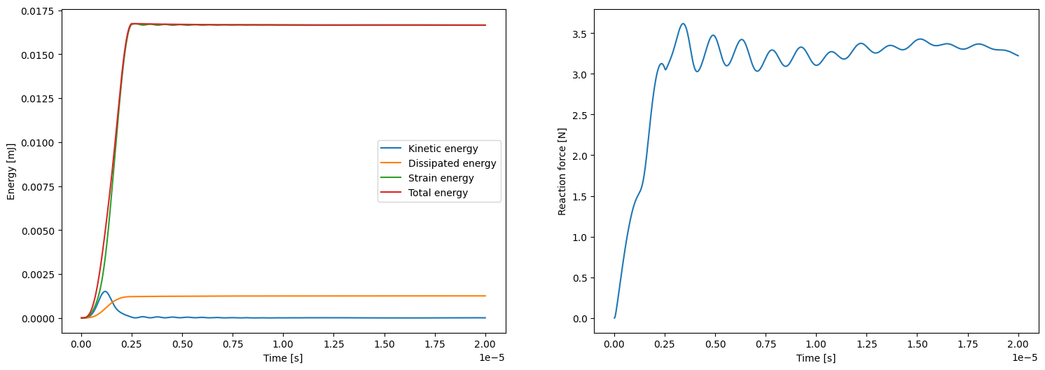
if comm.rank == 0:
fig2, ax2 = plt.subplots(1, 2, figsize=(18,6))
ax2[0].plot(ts, kinetic_energies, label='Kinetic energy')
ax2[0].plot(ts, dissipated_energies, label='Dissipated energy')
ax2[0].plot(ts, elastic_energies, label='Strain energy')
ax2[0].plot(ts, kinetic_energies + elastic_energies, label='Total energy')
ax2[0].set_xlabel('Time [s]')
ax2[0].set_ylabel('Energy [mJ]')
ax2[0].legend()
ax2[1].plot (ts, reaction_force_right_s)
ax2[1].set_xlabel('Time [s]')
ax2[1].set_ylabel('Reaction force [N]')
plt.show()
[output:0]