Mesh generation and visualization#
Authors: Corrado Maurini (corrado.maurini@sorbonne-universite.fr)
In this notebook you will find examples to
Generate meshes with
gmshand import them indolfinxVisualize the
dolfinxmesh directly in the notebook usingpyvistaSave the mesh to an
xdmffile
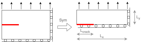
We consider an elastic slab \(\Omega\) with a straight crack \(\Gamma\) Using the symmetry, we will consider only half of the domain in the computation and we refine the mesh around the crack tip.
Let us generate a mesh using gmsh (http://gmsh.info/).
The function to generate the mesh is reported in the external file meshes.py.
The mesh is refined around the crack tip.
import gmsh
import numpy as np
from mpi4py import MPI
from dolfinx.io import gmsh as gmshio
import dolfinx.plot
We define below the geometrical parameters of the mesh.
Lx = 1.0
Ly = 0.5
Lcrack = 0.3
lc = 0.1
dist_min = 0.1
dist_max = 0.3
refinement_ratio = 10
gdim = 2
The following code block generates the mesh using the gmsh python interface. We refer the reader to the gmsh documentation for details: https://gmsh.info/doc/texinfo/gmsh.html
We also define MPI communicators, which are required only in parallel computation.
They are not strictly necessary here, but we keep them to have this example working in general.
The are set so that when we perform parallel computations, the mesh is generated on one processor (model_rank=0) and then it is distributed to all the processors (mesh_comm = MPI.COMM_WORLD). Further documentation about the use of MPI can be found at https://scientificcomputing.github.io/mpi-tutorial/notebooks/dolfinx_MPI_tutorial.html
We define a dictionary tags to associate clear names to numerical tags that are used to identify the different parts of the domain and the boundary
mesh_comm = MPI.COMM_WORLD
model_rank = 0
gmsh.initialize()

facet_tags = {"left": 1, "right": 2, "top": 3, "crack": 4, "bottom_no_crack": 5}
cell_tags = {"all": 20}

if mesh_comm.rank == model_rank:
    model = gmsh.model()
    model.add("Rectangle")
    model.setCurrent("Rectangle")
    # Create the points
    p1 = model.geo.addPoint(0.0, 0.0, 0, lc)
    p2 = model.geo.addPoint(Lcrack, 0.0, 0, lc)
    p3 = model.geo.addPoint(Lx, 0, 0, lc)
    p4 = model.geo.addPoint(Lx, Ly, 0, lc)
    p5 = model.geo.addPoint(0, Ly, 0, lc)
    # Create the lines
    l1 = model.geo.addLine(p1, p2, tag=facet_tags["crack"])
    l2 = model.geo.addLine(p2, p3, tag=facet_tags["bottom_no_crack"])
    l3 = model.geo.addLine(p3, p4, tag=facet_tags["right"])
    l4 = model.geo.addLine(p4, p5, tag=facet_tags["top"])
    l5 = model.geo.addLine(p5, p1, tag=facet_tags["left"])
    # Create the surface
    cloop1 = model.geo.addCurveLoop([l1, l2, l3, l4, l5])
    surface_1 = model.geo.addPlaneSurface([cloop1])

    # Define the mesh size and fields for the mesh refinement
    model.mesh.field.add("Distance", 1)
    model.mesh.field.setNumbers(1, "NodesList", [p2])
    # SizeMax -                   / ------------------
    #                            /
    # SizeMin -o----------------/
    #          |                |  |
    #        Point        DistMin   DistMax
    model.mesh.field.add("Threshold", 2)
    model.mesh.field.setNumber(2, "IField", 1)
    model.mesh.field.setNumber(2, "LcMin", lc / refinement_ratio)
    model.mesh.field.setNumber(2, "LcMax", lc)
    model.mesh.field.setNumber(2, "DistMin", dist_min)
    model.mesh.field.setNumber(2, "DistMax", dist_max)
    model.mesh.field.setAsBackgroundMesh(2)
    gmsh.option.setNumber("General.Verbosity", 3)
    model.geo.synchronize()

    # Assign mesh and facet tags
    surface_entities = [entity[1] for entity in model.getEntities(2)]
    model.addPhysicalGroup(2, surface_entities, tag=cell_tags["all"])
    model.setPhysicalName(2, 2, "Rectangle surface")
    model.mesh.generate(gdim)

    for key, value in facet_tags.items():
        model.addPhysicalGroup(1, [value], tag=value)
        model.setPhysicalName(1, value, key)
We can now import the mesh in dolfinx
msh, cell_tags, facet_tags, *_ = gmshio.model_to_mesh(
    model, mesh_comm, model_rank, gdim=gdim
)
msh.name = "rectangle"
cell_tags.name = f"{msh.name}_cells"
facet_tags.name = f"{msh.name}_facets"
with dolfinx.io.XDMFFile(MPI.COMM_WORLD, "output/mesh.xdmf", "w") as file:
    file.write_mesh(msh)
    msh.topology.create_connectivity(1, 2)
    file.write_meshtags(cell_tags, msh.geometry)
    file.write_meshtags(facet_tags, msh.geometry)
To plot the mesh we use pyvista see:
https://jorgensd.github.io/dolfinx-tutorial/chapter3/component_bc.html
https://docs.fenicsproject.org/dolfinx/main/python/demos/pyvista/demo_pyvista.py.html
import pyvista

pyvista.set_jupyter_backend("static")


# Extract topology from mesh and create pyvista mesh
topology, cell_types, x = dolfinx.plot.vtk_mesh(msh)
grid = pyvista.UnstructuredGrid(topology, cell_types, x)

plotter = pyvista.Plotter()
plotter.add_mesh(grid, show_edges=True)
plotter.camera_position = "xy"

if not pyvista.OFF_SCREEN:
    plotter.show()
else:
    plotter.screenshot("mesh.png")
2026-07-27 09:10:16.167 ( 0.473s) [ 7FAFE2DD1140]vtkXOpenGLRenderWindow.:1460 WARN| bad X server connection. DISPLAY=
We wrap the code to generate the mesh in the external module ../python/meshes to reuse it in the following tutorials.
We can use it as follows:
import sys

sys.path.append("../utils")
from meshes import generate_mesh_with_crack

msh, mt, ft = generate_mesh_with_crack(
    Lcrack=Lcrack,
    Ly=0.5,
    lc=0.1,  # caracteristic length of the mesh
    refinement_ratio=10,  # how much it is refined at the tip zone
    dist_min=dist_min,  # radius of tip zone
    dist_max=dist_max,  # radius of the transition zone
    verbosity=5,
)
Info    : Meshing 1D...
Info    : [  0%] Meshing curve 1 (Line)
Info    : [ 30%] Meshing curve 2 (Line)
Info    : [ 50%] Meshing curve 3 (Line)
Info    : [ 70%] Meshing curve 4 (Line)
Info    : [ 90%] Meshing curve 5 (Line)
Info    : Done meshing 1D (Wall 0.00255948s, CPU 0.002903s)
Info    : Meshing 2D...
Info    : Meshing surface 1 (Plane, Frontal-Delaunay)
Info    : Done meshing 2D (Wall 0.00624545s, CPU 0.006255s)
Info    : 413 nodes 829 elements
Warning : Gmsh has aleady been initialized